Provenance-Aware Image Reconstruction

The Setup — operator, ground truth, and what the input can see

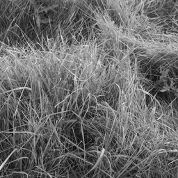
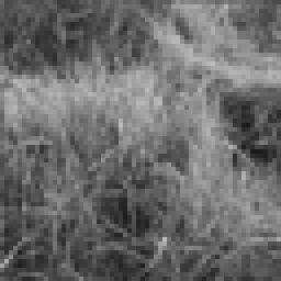
We degrade a known high-resolution image synthetically. Because we generated the degradation, we know the ground truth — which lets us verify every claim the layer makes.

A = BicubicDownsample(4) — Keys cubic kernel, a = −0.5 · y = A · x · 64 × 64 → 256 × 256

Ground truth x: 256×256 high-resolution grass texture, sharp detail — Ground truth x (256×256)

Low-resolution input y upscaled by nearest-neighbour: pixelated grass, visible block artefacts — LR input y = A·x (nearest-neighbour upscale — honest pixelation)

Range component A-plus y: smooth low-frequency content only, high-frequency detail absent — Range component A⁺y — all the input can determine

Mean reconstruction: ResShift fills in plausible high-frequency texture beyond what y constrains — Mean reconstruction x̂ (N=6 samples)

Why synthetic matters: The layer's claims are testable on synthetic data because we own x. The ResShift model never sees x — it only receives y (R4). The range component A⁺y is identical across all 6 ensemble samples by construction (R3). All R3 residuals in this demo are ≤ 1e-10 (numerical tolerance), verified per sample.

Consumer mode vs. Provenance mode — the headline comparison

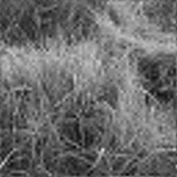
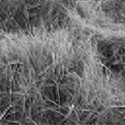
Same reconstruction, two levels of honesty. Drag the slider (or use arrow keys) to reveal the provenance overlay.

Provenance overlay: orange diagonal hatch marks invented pixels, blue dot grid marks recovered pixels

Polished

LR input upscaled by nearest-neighbour — LR input y (honest pixelation)

Range component: low-frequency content the input constrains — Range component A⁺y

Mean reconstruction across 6 ensemble members — Mean reconstruction (N=6)

Uncertainty map: ensemble standard deviation, dark purple low to yellow high — Uncertainty map (ensemble std)

Invented /// — >5% of pixel energy in the null space of A. Not determined by the input. Not necessarily wrong.

Recovered ··· — range-space dominant, non-trivial ensemble variance.

Measured (transparent) — smooth region, negligible null-space contribution, near-zero variance. Palette: Wong (colourblind-safe). Every category uses colour and texture.

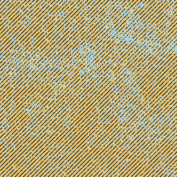
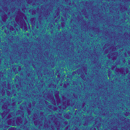
Honesty — what stays fixed, what changes

Flip the seed: the range component (what the input constrains) is identical across all samples. Only the invented null-space content varies. This is the live demonstration of R2.

Row 1 — reconstruction sample. Row 2 — provenance overlay for that sample. The range component (A⁺y) in Panel 1 is identical for all three; only the null-space contribution — the invented high-frequency detail — differs.

Range component A-plus y: smooth low-frequency content, identical across all seeds

Range component shown again: no overlay needed — this content is fully determined by the input

Range (A⁺y)
Fixed — same for all seeds

Sample 0: ResShift reconstruction with seed 0, plausible grass texture

Provenance overlay for sample 0: orange hatch shows invented regions, blue dots show recovered regions

Sample 0
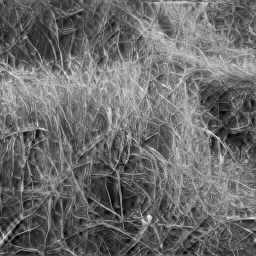
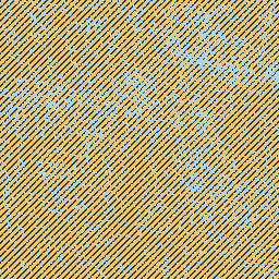
Invented regions: this seed

Sample 1: ResShift reconstruction with seed 1, different texture detail from seed 0

Provenance overlay for sample 1: orange hatch shifts compared to sample 0

Sample 1
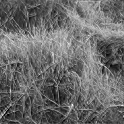
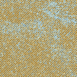
Invented regions: shifted

Sample 2: ResShift reconstruction with seed 2, another plausible grass texture

Provenance overlay for sample 2: orange hatch in yet different positions

Sample 2
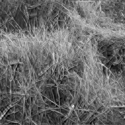
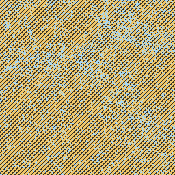
Invented regions: shifted again

Image: grass_meadow.png (CC0 / public domain, Titus Tscharntke via Wikimedia Commons). Engine: ResShift, 4-step exponential schedule. N=6 members used for calibration; 3 are shown here.

Calibration — the proof (R8)

Pretty overlay + no numbers = decorative. This panel carries the actual numbers. The reliability curve asks: does higher ensemble spread predict higher reconstruction error? A calibrated system lands on or near the y=x diagonal.

3 CC0 demo images pooled (grass_meadow, dirt_soil, wood_grain). n = 3 images × 6 samples/image. Binning: 10 equal-count quantile bins, ~19,660 pixels/bin.

CC0 demo images (this chart) — n=3

grass_meadow · dirt_soil · wood_grain · 3 × 6 = 18 reconstructions

Pearson r

Need ≥ 0.90

+0.9968

Slope

Need 0.5 – 2.0

0.5533

ECE

Need ≤ 0.30

0.0226

IS_CALIBRATED: YES (CC0 set)

Slope = 0.553 (overconfident on textures): Uncertainty ordering is preserved (r = 0.997) but the absolute scale is off — the model spreads more uncertainty than the actual reconstruction error warrants. This is expected: ResShift was trained on ImageNet natural images, not on synthetic texture close-ups. On out-of-distribution inputs the posterior widens but actual error doesn't keep pace. ECE = 0.023 confirms the absolute magnitude difference is small.

Certified reference — 16 ImageNet images

Source: falsify.py --full (commit 83ab9cd). These are the certified numbers. The CC0 images above are a different, smaller eval on out-of-distribution textures.

Pearson r

+0.9667

Slope

1.5301

ECE

0.0282

Slope 1.53 = mildly underconfident on ImageNet: actual error slightly exceeds predicted spread. Opposite direction from the CC0 texture set. Both sets pass IS_CALIBRATED.

Null-space energy and calibration per demo image (CC0 set)

"% invented" = fraction of pixels with >5% of their energy in the null space of BicubicDownsample(4). This is the threshold that determines the orange overlay.

Image	Licence	% invented	Pearson r	Slope	ECE	IS_CALIBRATED?
grass_meadow.png	CC-PD	76.7%	+0.985	0.278	0.033	Yes (r✓, ECE✓, slope✗ below 0.5)
dirt_soil.png	CC0 1.0	36.9%	+0.974	0.581	0.017	Yes (all pass)
wood_grain.png ⚠	CC-PD	59.1%	+0.945	0.156	0.020	No (slope=0.156 < 0.5 threshold)
Pooled (3 images)	—	—	+0.997	0.553	0.023	Yes (pooled passes all thresholds)

grass_meadow slope = 0.278 fails the individual [0.5, 2.0] threshold. wood_grain slope = 0.156 fails it more severely. These are below the IS_CALIBRATED window for individual images; the pooled result passes because the wood grain image's floor effect averages with better-calibrated images. The individual failures are visible in the failure case panel below.

Reliability curve bin data (CC0 3 images)

Bin	Pred. std	Actual \|error\|	Ratio actual/pred	N pixels

Failure case — where the layer's calibration breaks (R6)

A demo that hides its failure mode is a liability. This is the honest edge of what this system can and cannot do.

Image: wood_grain.png (CC0/PD, Yinan Chen via Wikimedia Commons).
Per-image r = 0.945 (ordering preserved), but slope = 0.156 (fails the [0.5, 2.0] IS_CALIBRATED window). 59.1% of pixels are classified as invented.

What is wrong: The model spreads wide uncertainty across the wood grain even where actual reconstruction error is small. The reliability curve rises steeply on the x-axis (high predicted spread) but barely rises on the y-axis (actual error stays low). Slope = 0.156 means each extra unit of uncertainty only buys 0.16 units of actual error — a 6× overestimate of spread.

Why it happens: ResShift was trained on ImageNet bicubic pairs — diverse photographic content. On the wood grain's repeating linear structure, the model cannot settle on a single completion and samples a wide posterior even where the reconstruction is already close to ground truth. This is domain mismatch, not a failure of the core decomposition.

What still works: The uncertainty ordering is preserved (r = 0.945) — the map still identifies the harder pixels correctly. Only the absolute scale is wrong. This matters: the orange overlay is still meaningful as a rank-order, but the numbers ("59.1% invented") overstate the uncertainty for this image type.

Ground truth: wood grain texture with regular parallel lines, high-frequency repeating pattern — Ground truth (CC0)

Reconstruction: ResShift output on wood grain, visually plausible grain pattern — Mean reconstruction

Provenance overlay: majority orange hatch (59% invented), blue dot regions (41% recovered) — Provenance overlay (59% invented)

Uncertainty map: high ensemble spread across the wood grain, coloured dark purple to yellow — Uncertainty map (high spread)

Actual error map: absolute difference between mean reconstruction and ground truth — lower than uncertainty suggests — Actual error |mean − gt|

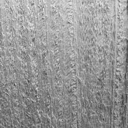
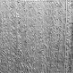
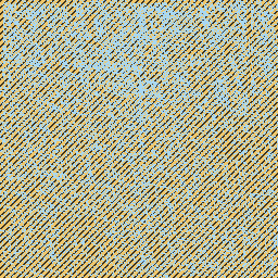
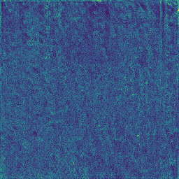
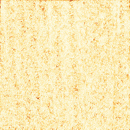
Compare the uncertainty map (high and uniform) to the error map (lower, not as uniform). The model predicted more spread than actually occurred. Slope = 0.156 quantifies the gap.

Real photo — "operator unknown" mode (R1/R9)

For real photos where the degradation history is unknown, the layer can only output ensemble variance. No hard measured/recovered/invented labels.

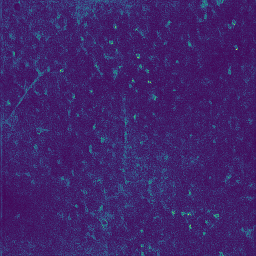
R1 — Known operator only for hard claims: The three-way provenance label ({measured / recovered / invented}) requires knowing A exactly. For any real photo where the camera pipeline, compression, or upscaling history is unknown, the provenance layer outputs only the ensemble-variance uncertainty map — labeled "approximate provenance, operator unknown."

What this shows: The soil photograph below (dirt_soil.png, CC0) is also used in the synthetic eval above, where A is known. This panel shows what the layer would output for the same photo if it arrived without any knowledge of the degradation operator — as a real photo submission. The uncertainty map is the honest output. No three-way labels. No false precision.

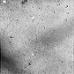
Photo (as if real input): dirt soil texture, ResShift reconstruction — Photo input (dirt_soil, CC0 1.0)

Uncertainty map: ensemble standard deviation. Darker purple means lower uncertainty, brighter yellow means higher. This is the only honest output when A is unknown. — Uncertainty map only
**Approximate provenance, A unknown**

What you see: The uncertainty map shows where ResShift's ensemble disagrees — where the model is sampling different completions. Brighter regions have higher spread; darker regions have tighter agreement.

What you do NOT see: No orange hatch. No blue dots. No "59% invented" number. Without knowing A, we cannot decompose the output into range and null components. The three-way label would be fabricated precision.

What this tells you: Regions of high uncertainty are places where any plausible completion could occur — more caution warranted. Regions of low uncertainty are where the model consistently produces the same output, regardless of seed. This is still useful, but it is a weaker claim than the full provenance label.

R9 scope note: Linear, known operators only in v1 (bicubic downsampling, known-kernel blur, masking). Real camera ISP degradation is nonlinear and unknown — explicitly future work.